Analysis across Multiple Images
Xiyu Peng
2025-04-17
Source:vignettes/articles/spleen_analysis.Rmd
spleen_analysis.RmdIn this tutorial, we will show how to apply SpaTopic to jointly identify topics across multiple images.
Set-up
We will work on 9 spleen tissue images and illustrate how to apply SpaTopic to multiple images to jointly identify topics. The dataset object can be downloaded from here, with original source from a Cell paper. This dataset includes nine images: three control normal BALBc spleens (BALBc 1-3) and six MRL/lpr spleens (samples 4-9) at varying disease stages—early (MRL 4-6), intermediate (MRL 7-8), and late (MRL 9) (Figure 5A). Using a 30-plex protein marker panel, the study identified 27 major splenic-resident cell types across the nine tissue images. We use the cell type annotation in the original paper.
x<-readRDS(file = "~/Documents/Research/github/SpaTopic_benchmarking/data/mouse_spleen_data/spleen_df.rds")
names(x)
#> [1] "BALBc-1" "BALBc-2" "BALBc-3" "MRL-4"   "MRL-5"   "MRL-6"   "MRL-7"
#> [8] "MRL-8"   "MRL-9"
We firstly prepare this dataset as the required input for SpaTopic. For multiple images, SpaTopic requires a list of data frames as input, each with columns
- image
- X
- Y
- type
You may add additional axis Z for 3D image.
select_column<-function(data){
  data_select<-as.data.frame(cbind(data$sample, data$sample.X, data$sample.Y, data$sample.Z, data$cluster))
  colnames(data_select)<-c("image","X","Y","Z","type") # we also save the coordinate on Z axis
  data_select$image<-gsub("-", ".", data_select$image)
  data_select
}
dataset<-lapply(x,select_column)
names(dataset) ## names of the 9 images
#> [1] "BALBc-1" "BALBc-2" "BALBc-3" "MRL-4"   "MRL-5"   "MRL-6"   "MRL-7"
#> [8] "MRL-8"   "MRL-9"
head(dataset[["BALBc-1"]]) ## df for the first image
#>     image    X    Y                Z             type
#> 1 BALBc.1 2392 5646 28.7234042553191 CD11c(+) B cells
#> 2 BALBc.1 3783 5471 33.5106382978723 CD11c(+) B cells
#> 3 BALBc.1 3790 9311 9.57446808510638 CD11c(+) B cells
#> 4 BALBc.1 2406 4963 19.1489361702128 CD11c(+) B cells
#> 5 BALBc.1 5182 2014 33.5106382978723 CD11c(+) B cells
#> 6 BALBc.1 5183 9421 28.7234042553191 CD11c(+) B cells
Note: The option for 3D image axis = "3D" is only
available in the current development version with this example. New
tutorial for SpaTopic on 3D images will come soon!
Run SpaTopic
Once we have prepared data, we can start to run SpaTopic with number
of topic = 6. The initialization may takes time, and you may run the
algorithm in parallel do.parallel = TRUE with multiple
cores n.cores = 8.
library(SpaTopic)
library(sf)
## NOT RUN, TAKES ABOUT 10~15 MIN across 9 images with single core.
system.time(gibbs.res<-SpaTopic_inference(dataset, ntopics = 6, sigma = 20, region_radius = 150, burnin = 1500))
save(gibbs.res,file = "~/Documents/Research/github/SpaTopic_benchmarking/data/mouse_spleen_data/gibbs.res.v2.rdata")
load(file = "~/Documents/Research/github/SpaTopic_benchmarking/data/mouse_spleen_data/gibbs.res.v2.rdata")Visualize the result
We will still use Seurat Package to help for visualization. First, let’s create a list of Seurat Object.
spleen_objects<-list()
library(Seurat)
for(i in names(x)){
  counts<-as.matrix(x[[i]][,c(2:30,34)])
  rownames(counts)<-1:nrow(counts) ### to avoid bug for mismatch
  subset<-CreateSeuratObject(counts = t(counts), assay = "protein")
  subset$X<-x[[i]]$sample.X
  subset$Y<-x[[i]]$sample.Y
  subset$cluster<-x[[i]]$cluster
  subset$sample<-x[[i]]$sample
  coords <- CreateFOV(
    data.frame(X = subset$X,Y = subset$Y),
    type = c("centroids"),assay = "protein"
  )
  i<-gsub("-", ".", i) # seurat package does not like -
  subset[[i]] <- coords
  spleen_objects[[i]]<-subset
}
We first plot the spatial distribution of 27 cell types across 9 images.
library(ggplot2)
library(patchwork)
p_celltype<-NULL
for (i in names(spleen_objects)){
  object<-spleen_objects[[i]]
  object$cluster<-as.factor(object$cluster)
  p_celltype[[i]]<-ImageDimPlot(object, fov = i, group.by = "cluster", axes = FALSE, dark.background = F,cols = "glasbey")  + ggtitle(i) +
      theme(legend.position = "right",
      plot.title = element_text(size = 10),
      plot.margin = margin(0, 0, 0, 0, "null")  # Reduce margins (top, right, bottom, left)
    )
}
wrap_plots(p_celltype,nrow = 3,guides = "collect") & NoLegend()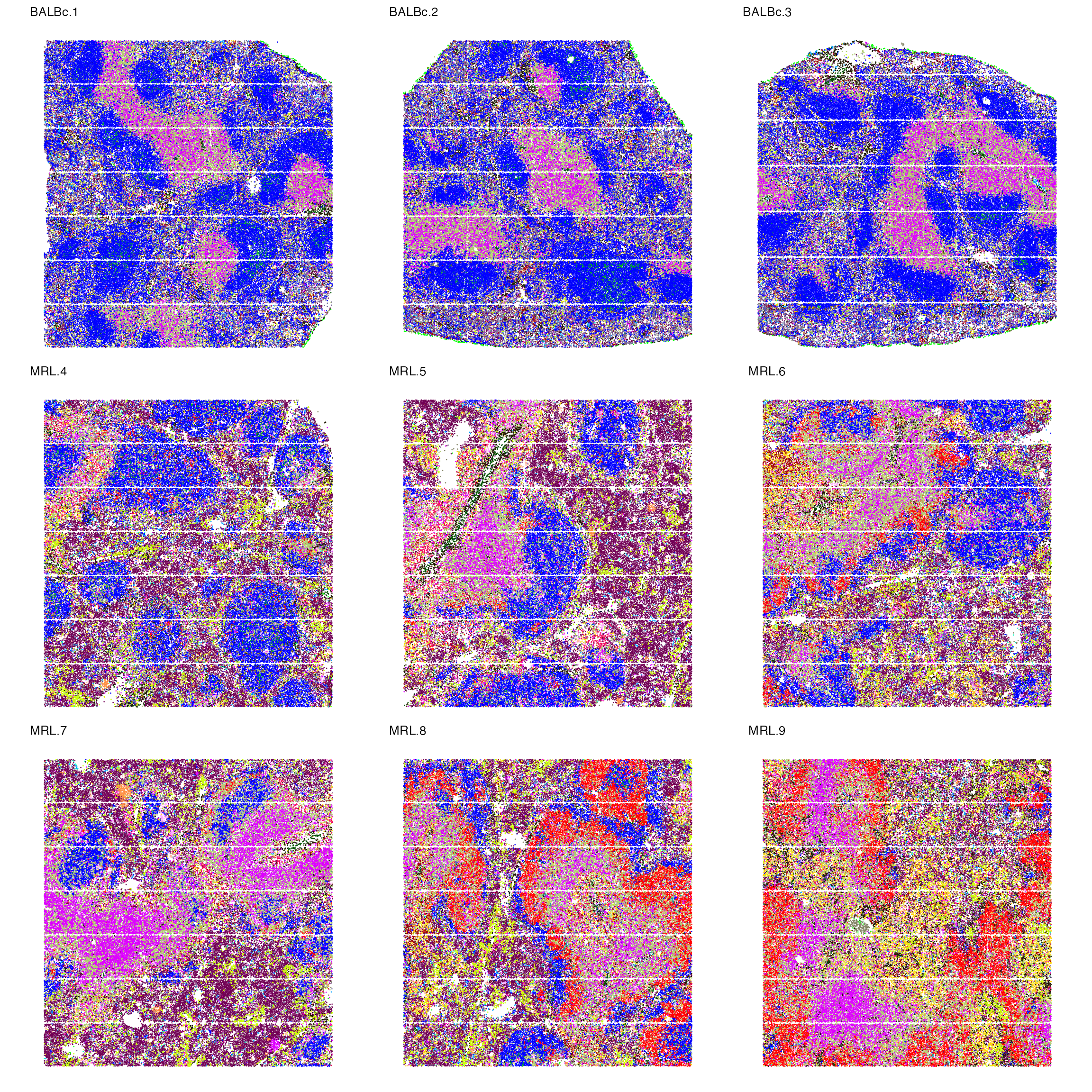
You may take a closer look on the first image
p_celltype[[1]]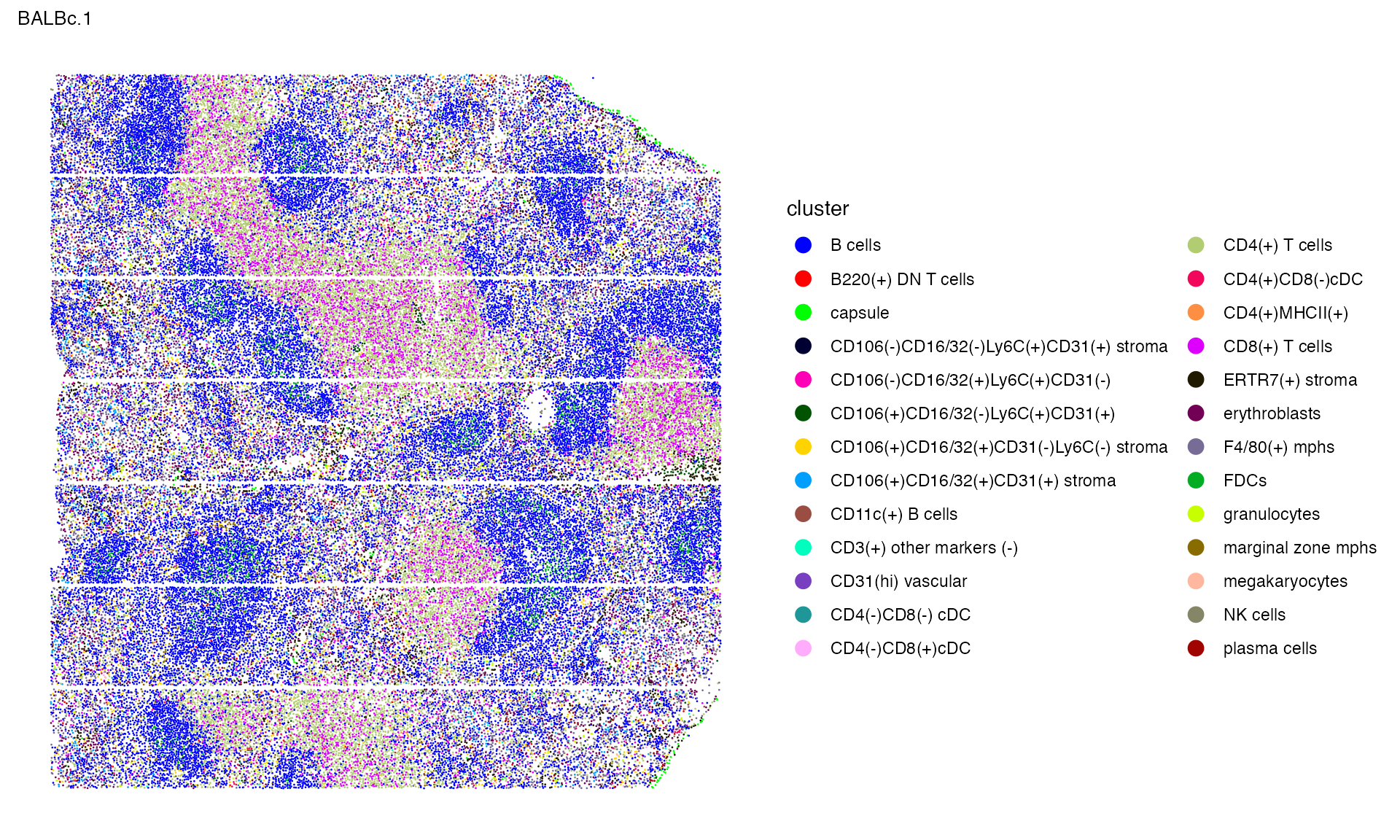
Then we add back the results from SpaTopic to the Seurat objects for visualization
itr_df<-do.call(rbind, dataset)
itr_df$image<-as.factor(itr_df$image)
itr_df$topic<-as.factor(gibbs.res$cell_topics)

## update result in seurat object
for(i in names(spleen_objects)){
    object<-spleen_objects[[i]]
    name2<-gsub("\\.", "-", i)
    object$Topic<-itr_df$topic[itr_df$image == i]
    spleen_objects[[i]]<-object
}
We also plot the spatial distribution of the main six topics.
palatte<- c("#0000FFFF","#FF0000FF","#00FF00FF","#009FFFFF","#FF00B6FF","#005300FF","#FFD300FF")
names(palatte)<-as.character(1:7)

p_spatopic<-NULL
for (i in names(spleen_objects)){
  object<-spleen_objects[[i]]
  object$Topic<-as.factor(object$Topic)
  p_spatopic[[i]]<-ImageDimPlot(object, fov = i, group.by = "Topic", axes = FALSE, dark.background = F,cols = palatte)  + ggtitle(i) +
      theme(legend.position = "right",
      plot.title = element_text(size = 10),
      plot.margin = margin(0, 0, 0, 0, "null")  # Reduce margins (top, right, bottom, left)
    )
}
wrap_plots(p_spatopic,nrow = 3,guides = "collect") & NoLegend()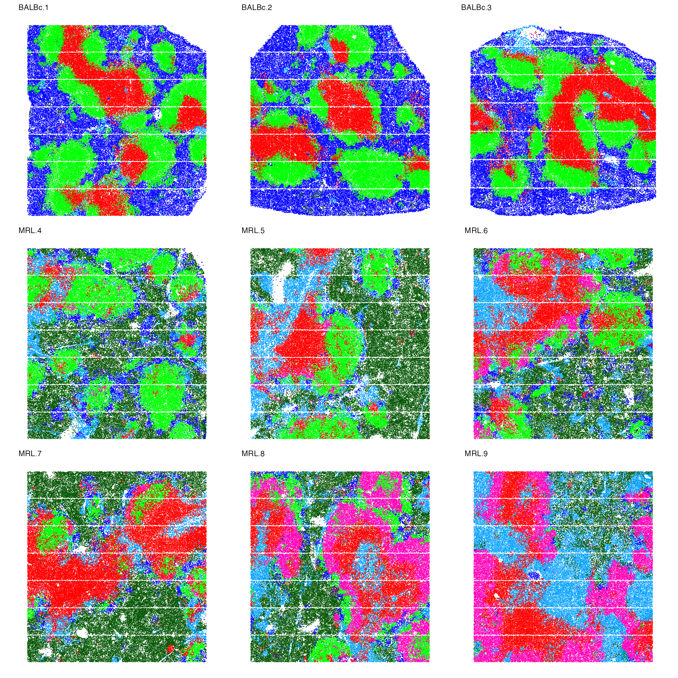
Let’s take a closer look on the first image again
p_spatopic[[1]]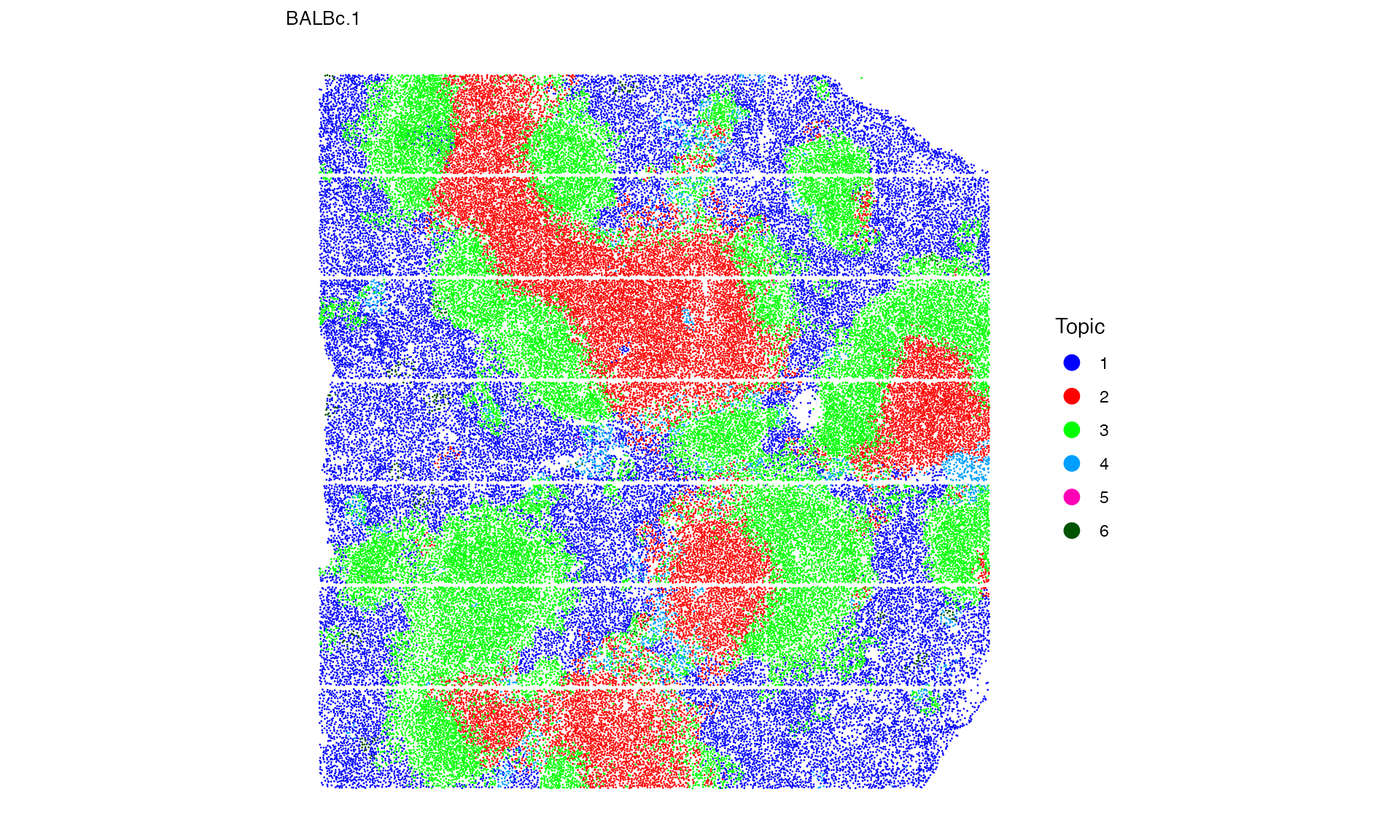
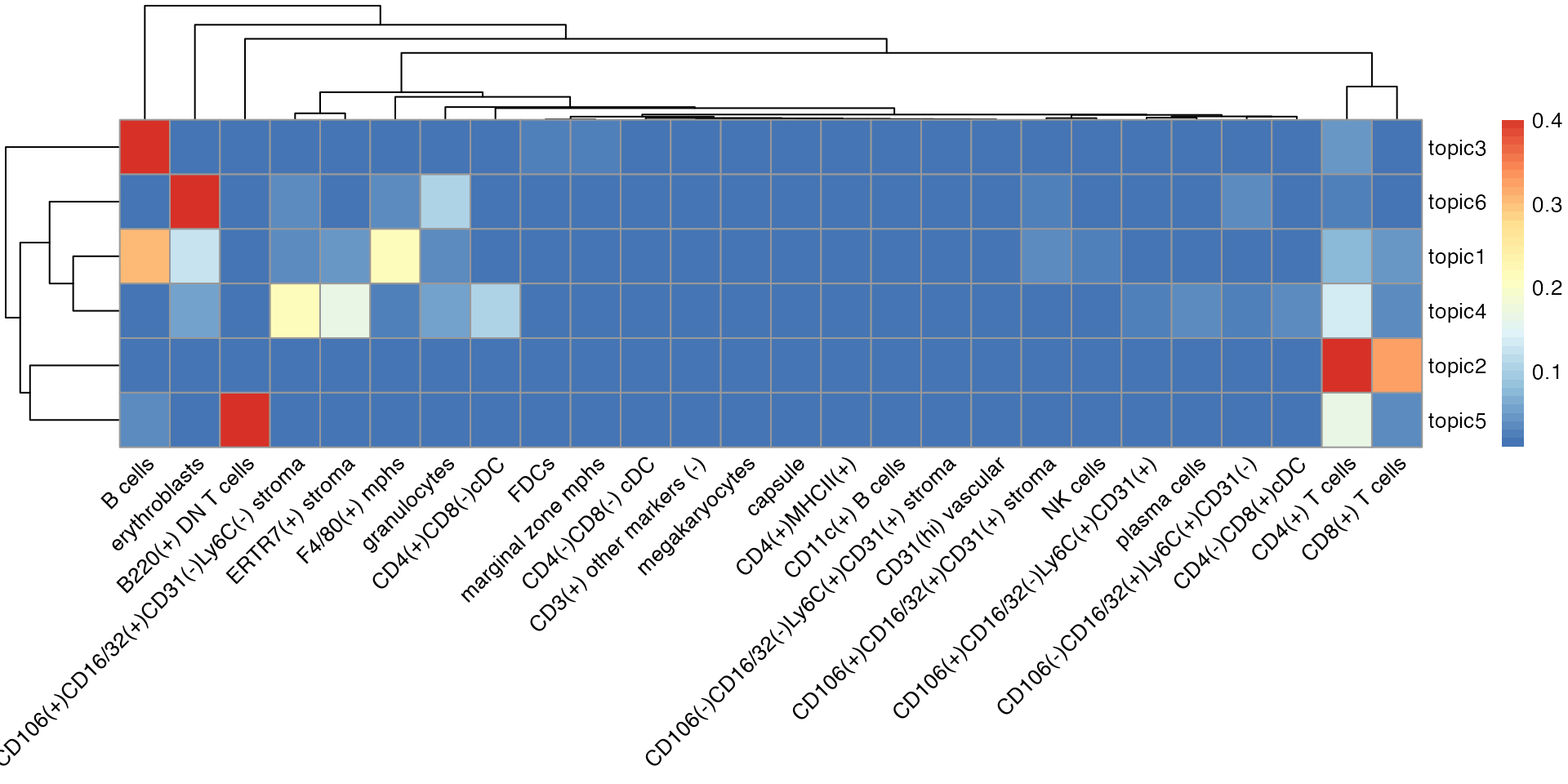
We use a heatmap to show the cell type distributions for all six topics:
- Normal spleen samples are primarily characterized by topics 1, 2, and 3, which reflect red pulp (mixed of B cells, erythroblasts, and F4/80(+) macrophages), PALS (mixed of CD8 T cells and CD4 T cells), and B-follicle (B cell dominated) respectively.
- There is an increase in Topic 6 and depletion of Topic 1 in MRL samples, representing much fewer B cells and F4/80(+) macrophages but more granulocytes and erythroblasts in the red pulp regions.
- Topic 5 (mainly B220(+) DN T cells and CD4(+) T cells) is enriched in lupus-affected spleen tissue at late stage.
m <- as.data.frame(gibbs.res$Beta)

library(RColorBrewer)
breaksList = seq(0.01, 0.4, by = 0.01)

# Plots the heatmap
pheatmap::pheatmap(t(m),
         color = colorRampPalette(rev(brewer.pal(n = 7, name = "RdYlBu")))(length(breaksList)),
         angle_col = 45,
         angle_row = 45,
         breaks = breaksList) # Sets the breaks of the color scale as in breaks List