Analysis for 3D image

NOTE: This tutorial is only for the development version of SpaTopic. Please install the latest version of SpaTopic from Github. It is not included in v1.2.0 on CRAN

devtools::install_github("xiyupeng/SpaTopic")

This is still under active development. We welcome any feedbacks.

Set up

library(SpaTopic)
packageVersion("SpaTopic")
#> [1] '1.2.0.9000'
library(sf)
#> Linking to GEOS 3.13.0, GDAL 3.8.5, PROJ 9.5.1; sf_use_s2() is TRUE

Again, we will work on a dataset of 9 spleen tissue images. We will focus on one image and illustrate how to use SpaTopic on a 3D image dataset. The dataset object can be downloaded from here, with original source from a Cell paper.

This dataset includes nine images: three control normal BALBc spleens (BALBc 1-3) and six MRL/lpr spleens (samples 4-9) at varying disease stages—early (MRL 4-6), intermediate (MRL 7-8), and late (MRL 9) (Figure 5A). Using a 30-plex protein marker panel, the study identified 27 major splenic-resident cell types across the nine tissue images. We use the cell type annotation in the original paper.

x<-readRDS(file = "~/Documents/Research/github/SpaTopic_benchmarking/data/mouse_spleen_data/spleen_df.rds")
names(x)
#> [1] "BALBc-1" "BALBc-2" "BALBc-3" "MRL-4"   "MRL-5"   "MRL-6"   "MRL-7"  
#> [8] "MRL-8"   "MRL-9"

We firstly prepare this dataset as the required input for SpaTopic. For multiple images, SpaTopic requires a list of data frames as input, each with columns

image
X
Y
Z (additional axis for 3D image)
type

Z should be the axis with the lowest range (max(Z) - min(Z)).

select_column<-function(data){
  data_select<-as.data.frame(cbind(data$sample, data$sample.X, data$sample.Y, data$sample.Z, data$cluster))
  colnames(data_select)<-c("image","X","Y","Z","type") # we also save the coordinate on Z axis
  data_select$image<-gsub("-", ".", data_select$image)
  data_select
}
dataset<-lapply(x,select_column)
names(dataset) ## names of the 9 images
#> [1] "BALBc-1" "BALBc-2" "BALBc-3" "MRL-4"   "MRL-5"   "MRL-6"   "MRL-7"  
#> [8] "MRL-8"   "MRL-9"
head(dataset[["BALBc-1"]]) ## df for the first image
#>     image    X    Y                Z             type
#> 1 BALBc.1 2392 5646 28.7234042553191 CD11c(+) B cells
#> 2 BALBc.1 3783 5471 33.5106382978723 CD11c(+) B cells
#> 3 BALBc.1 3790 9311 9.57446808510638 CD11c(+) B cells
#> 4 BALBc.1 2406 4963 19.1489361702128 CD11c(+) B cells
#> 5 BALBc.1 5182 2014 33.5106382978723 CD11c(+) B cells
#> 6 BALBc.1 5183 9421 28.7234042553191 CD11c(+) B cells

Running SpaTopic on 3D image

SpaTopic now supports full 3D spatial analysis, allowing you to leverage the complete spatial information in your tissue images. To enable 3D analysis, simply set axis = "3D" in the SpaTopic_inference function.

How it works? The package considers spatial relationships between cells in all three dimensions (X, Y, and Z), where Z represents the depth axis. For thick tissue sections, we implemented an adaptive sampling strategy that selects anchor cells across Z planes. The sampling density along the Z axis is controlled by the z_cellsize parameter, which we recommend setting to twice the region_radius by default.

Note that the Z axis should be the dimension with the smallest range (max(Z) - min(Z)) in your coordinate system.

For this image, we set ntopics = 4, similar as in the paper with four domains:

B-zone, marginal zone, PALS, red pulp

image1<-dataset[["BALBc-1"]]
system.time(gibbs.res<-SpaTopic_inference(image1, ntopics = 4, sigma = 20, region_radius = 150, burnin = 1500, axis = "3D"))
#> [11:49:04] [SpaTopic INFO] Number of cells per image: 81695
#> [11:49:04] [SpaTopic INFO] Start initialization...
#> [11:49:04] [SpaTopic INFO] Number of Initializations: 10
#> [11:49:19] [SpaTopic RESULT] Min perplexity during initialization: 4.5152
#> [11:49:19] [SpaTopic INFO] Number of region centers selected: 997
#> [11:49:19] [SpaTopic INFO] Average number of cells per region: 81.94
#> [11:49:19] [SpaTopic PROGRESS] Initialization complete. Starting Gibbs sampling...
#> [11:49:56] [SpaTopic COMPLETE] Gibbs sampling completed successfully
#> [11:49:56] [SpaTopic RESULT] Final model perplexity: 4.4702
#>    user  system elapsed 
#>  51.881   0.174  52.383

spleen_objects<-list()
library(Seurat)
for(i in names(x)){
  counts<-as.matrix(x[[i]][,c(2:30,34)])
  rownames(counts)<-1:nrow(counts)  ### to avoid bug for mismatch
  subset<-CreateSeuratObject(counts = t(counts), assay = "protein")
  subset$X<-x[[i]]$sample.X
  subset$Y<-x[[i]]$sample.Y
  subset$cluster<-x[[i]]$cluster
  subset$sample<-x[[i]]$sample
  coords <- CreateFOV(
    data.frame(X = subset$X,Y = subset$Y),
    type = c("centroids"),assay = "protein"
  )
  i<-gsub("-", ".", i) # seurat package does not like -
  subset[[i]] <- coords
  spleen_objects[[i]]<-subset
}

spleen_objects[["BALBc.1"]]$Topic_3D<-as.factor(gibbs.res$cell_topics)
ImageDimPlot(spleen_objects[["BALBc.1"]], fov = "BALBc.1", group.by = "Topic_3D", axes = FALSE, dark.background = F)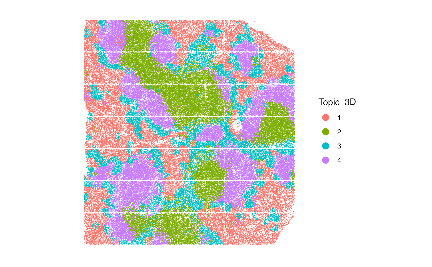

Visualize result in 3D

With the help with R package rgl, we are able to visualize the topic distribution in 3D.

library(rgl)
palatte<- c("#F8766D","#7CAE00","#00BFC4","#C77CFF")
names(palatte)<-as.character(1:4)

image_data<-dataset[["BALBc-1"]]
image_data$color <- palatte[spleen_objects[["BALBc.1"]]$Topic_3D]

plot3d( 
  x=image_data$X, y=image_data$Y, z=image_data$Z, 
  col = image_data$color, 
  xlab="X", ylab="Y", zlab="Z")

rglwidget()

Xiyu Peng

2025-07-15

Set up

Running SpaTopic on 3D image

Visualize result in 3D